Table of Contents
Regression models are essential tools in data analysis, helping us understand relationships between variables and make accurate predictions. Whether in business, healthcare, finance, or science, regression models provide insights that drive informed decisions, reveal trends, and support strategic planning. By choosing the appropriate regression technique, analysts can enhance the reliability of their predictions and uncover complex patterns in data.
In this article, we’ll dive into what a regression model is, explore its various types and applications, and provide guidance on selecting the most suitable model for different scenarios. We will be using the Python scikit-learn library to provide basic starter codes for each type of regression, helping you get hands-on with the implementation of these models.
Key Terms Explained
Before diving into the regression techniques, let’s clarify some key terms that are essential for understanding the concepts and techniques discussed in this article.
1. Independent Variable
An independent variable is a feature or input used to predict the outcome. In the context of regression, these are the variables that drive changes in the dependent variable. For example, in predicting house prices, features like location, square footage, and number of bedrooms are independent variables.2. Dependent Variable
The dependent variable is the outcome or target we aim to predict. It is dependent on the values of the independent variables. For instance, the house price in the example above is the dependent variable.3. Overfitting
Overfitting occurs when a model learns the noise or random fluctuations in the training data instead of the true underlying patterns. While the model performs exceptionally well on training data, it fails to generalize to unseen data, resulting in poor performance on new datasets.
Example: A highly complex model predicting exact values for training data but struggling with new examples.4. Bias
Bias refers to the error introduced by assuming a simplified model to represent the underlying data. High bias leads to underfitting, where the model fails to capture the complexity of the data.
Example: A linear regression model attempting to fit data with a nonlinear relationship.5. Variance
Variance is the error introduced due to the model’s sensitivity to small fluctuations in the training data. High variance leads to overfitting, where the model captures noise as if it were a true pattern.
Example: A decision tree with no restrictions on depth fitting every detail of the training data.6. Multicollinearity
Multicollinearity arises when two or more independent variables in a regression model are highly correlated, making it difficult to determine the individual effect of each variable. This can lead to unstable predictions and reduced interpretability.
Example: In a housing price model, features like “size in square feet” and “number of rooms” may overlap in information.7. Regularization
Regularization is a technique used to prevent overfitting by adding a penalty term to the cost function. This helps reduce the model’s complexity and improves generalizability. Ridge regression and Lasso regression are common types of regularization techniques in regression analysis.
Example: Ridge regression penalizes large coefficients to prevent the model from fitting noise in the data.8. Supervised Learning
Supervised learning trains a model on labeled data, where each input is paired with a known output. The model learns to predict the output for new inputs by identifying patterns in the training data. It is used for tasks like regression (predicting continuous values) and classification (categorizing data).9. Unsupervised Learning
Unsupervised learning analyzes unlabeled data to identify patterns or groupings without predefined outcomes. It is used for tasks like clustering (grouping similar data points) and dimensionality reduction (simplifying data features).Understanding these terms will help you grasp the nuances of each regression method and make informed decisions when selecting the right technique for your data.
What is a Regression Model?
A regression model is a statistical tool that describes the relationship between one or more independent variables and the dependent, or target variable. By establishing this relationship, regression models allow us to predict outcomes, understand trends, and analyze the effect of various factors on a target variable. For instance, a linear regression model might capture the relationship between height and weight, providing a formula to predict weight based on height.
Regression analysis is widely used across fields, from finance to big data and scientific research, serving as a foundation for various predictive models. It is often behind studies that assess trends and impacts, such as fuel efficiency, pollution causes, or the effects of screen time on learning. In each of these cases, regression models help quantify the relationship between key variables, supporting conclusions with data-driven insights.
When to use it?
Regression models are invaluable tools when you need to analyze the relationship between variables and make predictions based on data. Here are some scenarios where regression models are particularly useful:
- Predicting Continuous Outcomes: Regression models are ideal when you want to predict continuous, numeric values. Examples include forecasting sales, estimating real estate prices, or predicting temperature changes based on historical data.
- Identifying Relationships Between Variables: Regression analysis is commonly used to understand how independent variables affect a dependent variable. For example, researchers might use regression to analyze how factors like age, income, or education level influence spending habits.
- Evaluating Trends and Patterns: In fields such as economics and finance, regression models help identify trends over time. For example, analyzing stock market performance based on interest rates or consumer spending trends can guide investment decisions.
- Assessing Impact in Experimental Studies: Regression models are often used in experimental and observational studies to quantify the impact of one variable on another, such as determining the effect of a new drug on health outcomes while controlling for factors like age and lifestyle.
- Supporting Decision-Making: Businesses and organizations use regression models to inform decisions by predicting outcomes under various scenarios. This is common in marketing, where regression can help forecast campaign success based on budget, audience demographics, and advertising channels.
Types of Regression
Regression models offer a diverse range of techniques, each tailored to handle specific data characteristics and types of relationships. Let’s go over some commonly used types of regression, illustrating how these techniques can be applied to real-world contexts to meet diverse prediction needs.
Linear Regression
Linear regression predicts the value of the dependent variable based on one or more independent variables. This is achieved by fitting a straight-line equation (or drawing a line of best fit) to observed data, making it highly effective at identifying patterns and trends in historical data.
For cases with more than one independent variable, multiple linear regression can be used to capture the combined effect of multiple factors, quantifying the main drivers of an outcome.
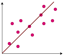
When to Use: Use linear regression when the relationship between the independent and dependent variables appears linear—meaning that a change in the independent variable results in a proportional change in the dependent variable. It is ideal for forecasting and trend analysis in scenarios where the relationship is stable and straightforward.
Examples:
- Estimating Housing Prices: Real estate companies can predict property prices based on characteristics like location, square footage, and age of the property.
- Forecasting Sales: Help a company project future sales by analyzing historical sales data alongside seasonal trends, marketing spend, and other relevant factors.
- Predicting Customer Churn: Use multiple linear regression to determine the factors that most impact customer churn rates, such as customer service interactions, account age, or monthly spending, helping companies take preventive actions.
Code
from sklearn.linear_model import LinearRegression
import numpy as np

# Sample data
X = np.array([[1], [2], [3], [4]])
y = np.array([2, 4, 6, 8])

# Model
model = LinearRegression()
model.fit(X, y)

# Prediction
pred = model.predict([[5]])
print("Prediction:", pred)
This example demonstrates simple linear regression, which predicts a continuous outcome based on a linear relationship with a single independent variable. The model is trained on sample data points, where X represents input values and y represents output values. After training, the model predicts the output for a new input (in this case, 5).
Logistic Regression
Logistic regression predicts binary or categorical outcomes using one or more independent variables. Unlike linear regression, which predicts continuous values, logistic regression estimates the probability of a specific event occurring, effectively classifying data into categories like true/false, 0/1, and yes/no.

When to Use: Logistic regression is ideal when you need to classify data into distinct categories or predict the probability of a binary event. It’s useful for cases where the outcome is categorical and not continuous, particularly when you want to make decisions based on the likelihood of an event occurring.
Examples:
- Predictive Maintenance in Manufacturing: Can estimate the probability of equipment failure based on factors like operating conditions, usage patterns, and historical data, enabling companies to proactively perform maintenance and reduce unexpected downtime.
- Customer Purchase Prediction: In e-commerce, it can help determine the likelihood of a customer making a purchase based on past browsing behavior, product preferences, and prior purchase history, guiding targeted marketing efforts.
- Healthcare Risk Assessment: Assess a patient’s likelihood of developing a particular condition, such as heart disease, by analyzing factors like age, lifestyle, medical history, and test results, supporting preventive care initiatives.
Code
from sklearn.linear_model import LogisticRegression

# Sample data
X = [[0], [1], [2], [3]]
y = [0, 0, 1, 1]

# Model
model = LogisticRegression()
model.fit(X, y)

# Prediction
pred = model.predict([[1.5]])
print("Prediction:", pred)
Here, logistic regression is used for binary classification, predicting if an outcome falls into one of two categories (e.g., true/false). The model is trained with input data, X, and binary labels, y, and can then classify new data points based on this training. In this example, the model predicts the category for an input value of 1.5.
Polynomial Regression
Polynomial regression models the relationship between dependent and independent variables as an nth-degree polynomial equation. By fitting a nonlinear curve to the data, it can effectively capture complex patterns and interactions that a linear model cannot. This makes it particularly valuable for analyzing data with curved trends and intricate relationships, such as those found in financial services, risk assessment, and predictive modeling.
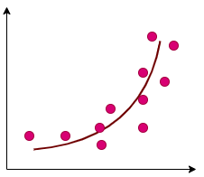
When to Use: Use polynomial regression when the relationship between variables is non-linear and cannot be adequately represented by a straight line. It is ideal for scenarios where the data exhibits a curved or intricate trend and requires a flexible model to capture the nuances.
Examples:
- Insurance Risk Assessment: Helps insurers assess risk by modeling nonlinear relationships between factors like age, driving history, and vehicle type, enabling more accurate underwriting decisions.
- Population Growth Modeling: In ecological studies, it can capture the growth rate of a population over time, which often follows a non-linear trajectory due to factors like resource availability and environmental constraints.
- Stock Market Analysis: Used in financial modeling to analyze trends in stock prices, capturing nonlinear patterns influenced by market dynamics, investor behavior, and economic indicators.
Code
from sklearn.preprocessing import PolynomialFeatures
from sklearn.linear_model import LinearRegression
import numpy as np

# Sample data
X = np.array([[1], [2], [3]])
y = np.array([1, 4, 9])

# Polynomial transformation
poly = PolynomialFeatures(degree=2)
X_poly = poly.fit_transform(X)

# Model
model = LinearRegression()
model.fit(X_poly, y)

# Prediction
pred = model.predict(poly.transform([[4]]))
print("Prediction:", pred)
In this example, polynomial regression captures nonlinear relationships by transforming the input data into polynomial terms before fitting a linear model. Here, a second-degree polynomial is used to model the data, and the model is trained on these transformed inputs. The model can then predict complex, nonlinear trends, as seen in the prediction for input 4.
Ridge Regression
Ridge regression is a regularized linear regression model. It is designed to handle datasets with multicollinearity, where independent variables are highly correlated. By adding a penalty term to the cost function, it reduces the magnitude of regression coefficients, effectively balancing bias and variance. This method prevents overfitting, improves the stability of the model, and ensures better predictive performance, especially in datasets with a large number of interrelated variables.
For cases where you want to simplify your model by automatically selecting a smaller subset of features, use Lasso regression; it introduces a penalty that can shrink coefficients to zero, effectively performing variable selection.
When to Use: Ridge regression is ideal when working with multiple regression data where multicollinearity is present. It is particularly useful for scenarios where standard linear regression models struggle due to high intercorrelations among independent variables, leading to unstable predictions.
Examples
- Disease Risk Prediction in Healthcare: Analyze the relationship between genetic, lifestyle, and environmental factors to predict an individual’s risk of developing diseases, providing reliable insights in complex, high-dimensional datasets.
- Marketing Campaign Analysis: It is used to evaluate the impact of various marketing channels (e.g., social media, email, advertisements) that exhibit multicollinearity, enabling marketers to allocate budgets more effectively.
- Predicting Housing Prices: Model the influence of interrelated factors like location, square footage, and amenities on housing prices, ensuring robust predictions even in the presence of multicollinearity.
Code
from sklearn.linear_model import Ridge
import numpy as np

# Sample data
X = np.array([[1], [2], [3]])
y = np.array([1, 4, 9])

# Model
model = Ridge(alpha=1.0)
model.fit(X, y)

# Prediction
pred = model.predict([[4]])
print("Prediction:", pred)
This example applies ridge regression, which penalizes large coefficients to prevent overfitting. Here, alpha controls the penalty’s strength, helping the model generalize better when features are highly correlated. The model is trained on sample data to predict a new value for input 4, aiming for stable predictions even in the presence of multicollinearity.
Decision Tree Regression
Decision Tree Regression is a supervised learning algorithm that models data using a tree-like structure. Each internal node represents a test on a feature, branches represent outcomes of the test, and leaf nodes provide the predicted continuous value. This non-parametric method is effective for handling both categorical and numerical data and capturing complex relationships.
When to use: Decision tree regression is used when the data exhibits non-linear relationships or when the dataset includes both categorical and numerical features. Additionally, decision trees are highly interpretable, making them ideal when a clear and transparent decision-making process is a priority, such as in cases where stakeholders need to understand how predictions are made.
Examples:
- House Price Prediction: Estimating house prices based on features like location, square footage, and number of bedrooms.
- Customer Spending Behavior: Predicting customer spending levels based on demographic and purchase history data.
- Agricultural Yield: Estimating crop yields based on factors such as rainfall, soil quality, and temperature.
Code
from sklearn.tree import DecisionTreeRegressor

# Sample data
X = [[1], [2], [3], [4]]
y = [2.5, 5, 7.5, 10]

# Model
model = DecisionTreeRegressor()
model.fit(X, y)

# Prediction
pred = model.predict([[3.5]])
print("Prediction:", pred)
This example uses a decision tree regressor to model data with potential non-linear relationships. The tree splits data at various levels, capturing complex patterns without requiring linearity. After training, the model can predict values for inputs within its learned splits; here, it predicts for 3.5, based on patterns from the training data.
Support Vector Regression
Support Vector Regression (SVR) is a regression technique derived from Support Vector Machines (SVM), designed to predict continuous output values. It works by finding a hyperplane that best fits the data while maintaining a margin within which most data points lie. SVR can utilize both linear and non-linear kernels, enabling it to handle simple as well as complex data patterns. The key components of SVR include the hyperplane for prediction, boundary lines that define margins, and support vectors—the data points closest to the hyperplane, which influence its position.
When to use: Support Vector Regression is ideal when the dataset contains both linear and non-linear patterns, requiring flexibility in modeling complex relationships. It excels in scenarios where the data includes outliers or noise, as the margin-based approach helps maintain robustness. Additionally, SVR is well-suited for small to medium-sized datasets where computational efficiency and precision are crucial.
Examples:
- Car Mileage Prediction: Estimating the mileage of a car based on features like engine size, weight, and fuel type.
- Crop Yield Forecasting: Predicting agricultural yield by analyzing soil quality, rainfall patterns, and temperature.
- Retail Sales Forecasting: Anticipating sales trends using factors such as seasonal demand, promotional activities, and economic conditions.
Code
from sklearn.svm import SVR

# Sample data
X = [[1], [2], [3], [4]]
y = [1.5, 3.5, 5.5, 7.5]

# Model
model = SVR(kernel='rbf', C=1.0, epsilon=0.2)
model.fit(X, y)

# Prediction
pred = model.predict([[3.5]])
print("Prediction:", pred)
This example demonstrates support vector regression, which fits a hyperplane within a defined margin to predict continuous outcomes. The model is flexible, with kernel functions that handle non-linear patterns. Here, SVR uses the radial basis function (RBF) kernel, fitting the model to the sample data to predict an outcome for input 3.5, balancing precision and robustness against outliers.
Each type of regression model has its strengths and is suited to different data types and relationships, allowing you to select the best approach based on the specific characteristics of your data and the nature of the predictions you want to make.
How to Create a Regression Model?
Creating a regression model involves a series of steps to define the problem, gather and explore data, select and train a model, and finally interpret the results. Here’s a breakdown of each step to guide you through the process:
Define the Problem
Identify what you want to predict or explain (the target or outcome variable). Then, determine the factors that might influence this outcome. These factors, or predictors, will become your independent variables in the model.
Gather Data
Collect relevant data that aligns with your problem and variables. This data could come from various sources, including databases, surveys, or historical records. Ensure that the data is clean and accurate, as missing or incorrect data can reduce the reliability of your model.
Explore the Data
Before building the model, examine the data for patterns or relationships between the independent variables and the outcome. Use visualizations like scatter plots or correlation matrices to assess how variables interact and to detect any initial patterns that could guide model selection.
Define Variables and Choose a Model
Define your variables clearly:
- Independent variables: Factors that you can control or measure that may influence the target.
- Dependent variable: The outcome or target variable you aim to predict.
This distinction is essential for setting up your model and interpreting the results. Then, based on your data and problem type, select an appropriate regression model. Use Linear Regression for relationships that appear linear, and logistic Regression for binary outcomes (e.g., yes/no). For complex scenarios with multiple factors, consider using advanced models like Multiple Regression or Polynomial Regression.
Plot the Data and Evaluate Correlations
Plot your data on graphs to visualize relationships between variables. A scatter plot is often used for single independent and dependent variables. If there appears to be a strong linear trend, this is a good indication that linear regression might fit well.
Train the Model
Split your data into a training set and a test set. Use the training set to teach the model how to recognize patterns and relationships in the data. By fitting the model to this data, it “learns” to make predictions based on these observed relationships.
Test the Model
Test your model using the test set to evaluate how accurately it predicts the target variable. This process checks whether the model generalizes well to new, unseen data, which is crucial for making reliable predictions.
Consider the Presence of Error
Recognize that no model is perfect; there will always be some degree of error in the predictions. Assessing this error is important to ensure the model’s reliability and accuracy.
Make Predictions and Interpret Results
Use the trained model to predict outcomes for new data. Review and interpret the results to understand how well the model aligns with real-world scenarios. Finally, analyze how the independent variables influence the dependent variable, which helps explain the practical significance of the model’s predictions.
By following these steps, you’ll create a regression model that not only fits your data well but also provides valuable insights into the relationships between variables and the factors influencing your target outcome.
Code Implementation
If you are confused about how to set up to run your regression model, don’t worry. We got you!
Running machine learning (ML) code requires an environment where you can write, execute, and test your algorithms. There are two main ways to do this: using cloud-based platforms like Google Colab or running code locally on your own machine. Let’s go through how you can run you code in both setups.
1. Running Machine Learning Code on Google Colab
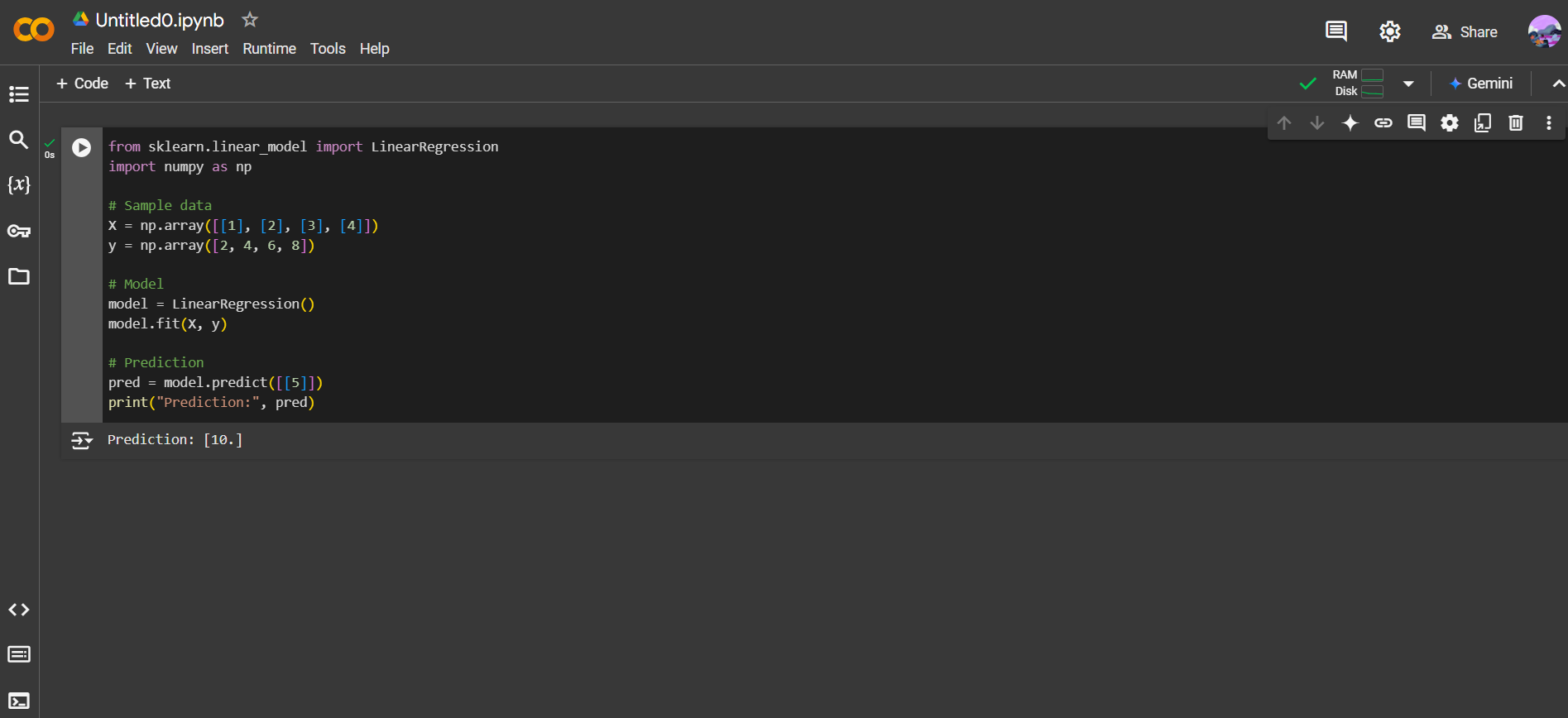
Google Colab is a free, cloud-based platform that provides an interactive environment for coding in Python, especially useful for machine learning. It gives access to powerful GPUs, which is ideal for training models on large datasets.
Access Google Colab: Open a browser. Go to Google Colab and sign in with your Google account.
Write or Paste Your ML Code: From the Runtime dropdown, select New notebook in Drive. Now, simply copy the code snippet given with each type of regression model into a cell in the notebook.
Run the Code: Colab runs code in cells. You can run each cell individually or execute all cells sequentially using the “Runtime” option at the top.
Use GPUs for Faster Computation: Google Colab offers free (but limited) access to GPUs as well. To enable GPU: Go to Runtime > Change runtime type and select GPU as the hardware accelerator.
Save and Share: You can save your work to Google Drive or download it as a .ipynb file.
Benefits of Google Colab:
- No installation required.
- Free access to GPUs and TPUs.
- Easy collaboration and sharing.
- Direct access to Google Drive for storing datasets.
2. Running Machine Learning Code Locally
Running machine learning code locally involves setting up a Python environment on your computer. This is ideal if you want more control over your machine’s resources and do not want to rely on cloud services.
Install Python: Download and install Python from python.org. It’s recommended to install Python 3.x, as it supports modern libraries.
Install Machine Learning Libraries: (You can first create a virtual environment to avoid future conflicts between different versions of libraries.) Use pip to install the required libraries:
pip install numpy pandas scikit-learn matplotlibWrite Your Code: Open a code editor like Visual Studio Code, Jupyter Notebook, or PyCharm. Create a new file regression_models.py and copy the code snippet given with each type of regression model into it.
Run the Code: In your terminal or IDE, you can run your Python scripts with the following command:
python3 regression_models.py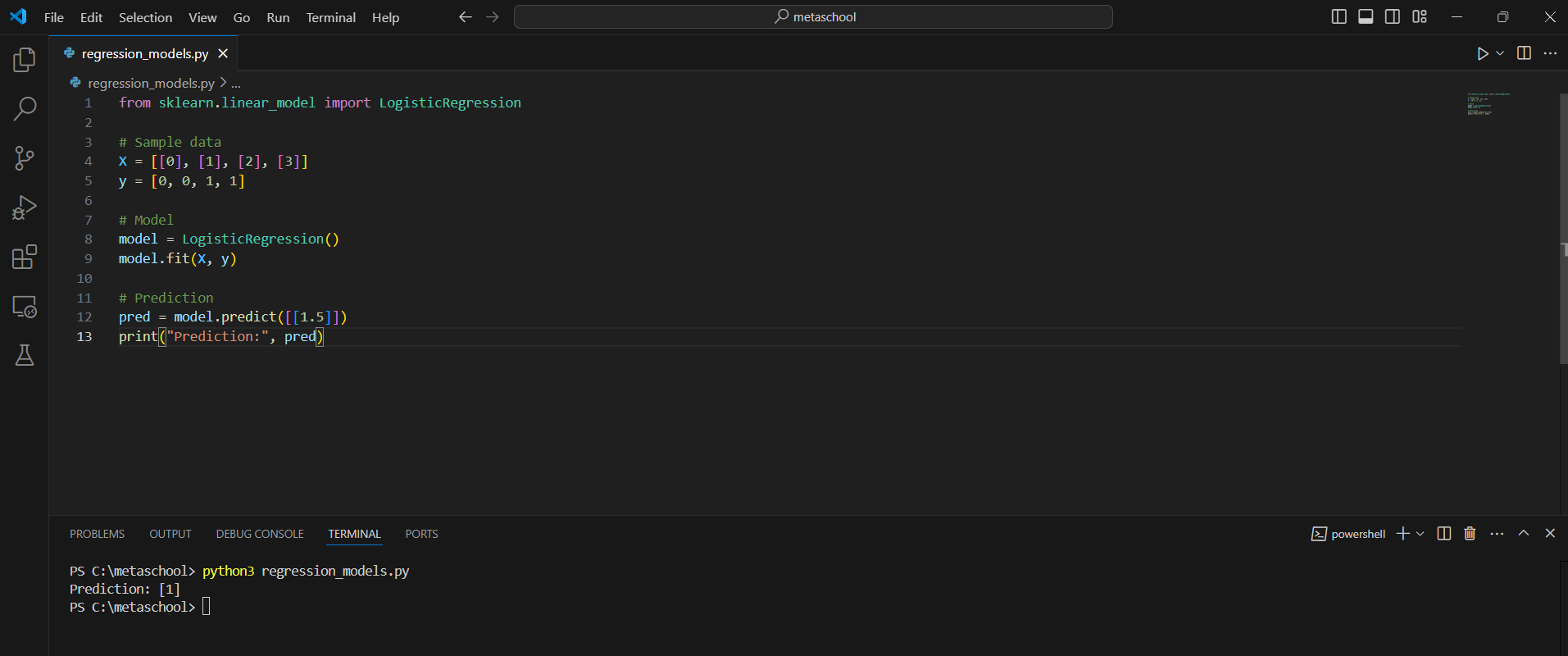
Benefits of Running ML Code Locally:
- Full control over your environment and data.
- No dependency on internet access.
- Better suited for custom setups with specific requirements (like hardware optimizations).
Conclusion
| Algorithm | When to Use |
|---|---|
| Linear Regression | Use when the relationship between independent and dependent variables is linear and straightforward. Ideal for forecasting and trend analysis. |
| Logistic Regression | Use when predicting binary or categorical outcomes. Suitable for classification problems like yes/no or true/false decisions. |
| Polynomial Regression | Use when the relationship between variables is nonlinear but can be modeled by polynomial functions. Ideal for curved trends. |
| Ridge Regression | Use when dealing with multicollinearity (high correlation among independent variables) to improve model stability. |
| Lasso Regression | Use when you want to perform feature selection by shrinking some coefficients to zero while reducing overfitting. |
| Decision Tree Regression | Use for non-linear relationships or when interpretability is important. Handles both numerical and categorical data well. |
| Support Vector Regression (SVR) | Use when the dataset contains linear or nonlinear patterns and requires robustness against noise or outliers. |
Regression is a cornerstone of predictive modeling, offering powerful techniques to uncover relationships and predict outcomes from data. However, for complex datasets, a single model may not always be sufficient. Combining multiple models or using advanced techniques can often yield better predictions. Additionally, good results depend not only on the choice of the algorithm but also on factors like data quality, availability, and proper preprocessing, such as data cleaning and feature engineering. By carefully considering these elements, you can create robust models that deliver meaningful insights and accurate predictions.
Related Reading:
- 10 Best Machine Learning Libraries (With Examples)
- What is the Mixture of Experts — A Comprehensive Guide
- What is RAG in AI – A Comprehensive Guide
- What is Generative AI, ChatGPT, and DALL-E? Explained
FAQs
What are the five types of regression models?
The five commonly used types of regression models are:
1. Linear Regression – Models a linear relationship between independent and dependent variables.
2. Logistic Regression – Used for binary classification, predicting probability outcomes.
3. Polynomial Regression – Fits a nonlinear relationship by transforming variables into a polynomial equation.
4. Ridge Regression – A type of linear regression with regularization to prevent overfitting by adding a penalty to the coefficients.
5. Lasso Regression – Another regularization method that performs feature selection by shrinking coefficients of less important features to zero.
What are the three regression models?
Three key types of regression models are:
Linear Regression – Best for relationships that follow a straight line.
Logistic Regression – Ideal for binary or categorical outcome predictions.
Polynomial Regression – Suitable for data where the relationship is curved or non-linear.
Why is it called a regression model?
The term “regression” originates from the work of Sir Francis Galton in the 19th century, who noticed that children’s heights tended to “regress” or move closer to the average height of the population. In statistics, regression models help “regress” or predict an outcome variable based on one or more predictor variables.
Which regression model is best?
The best regression model depends on the data and the relationship between variables. Linear regression works well for linear relationships, logistic regression is optimal for binary outcomes, and polynomial regression fits non-linear data. Regularized models like ridge or lasso regression are preferable when overfitting is a concern.
