
Table of Contents
In the world of AI and ML, linear regression is one of the most fundamental and widely used tools. It’s often the first algorithm aspiring data scientists and AI enthusiasts learn, and for good reason. Linear regression is not just a stepping stone to more complex models—it’s a powerful technique in its own right, with applications spanning industries like finance, healthcare, marketing, and beyond. From predicting house prices to forecasting sales, linear regression helps us uncover patterns in data and make informed decisions.
In this article, we will discuss what linear regression is, how it works, and some real-world use cases. We will also look at how you can implement it using built-in libraries in Python.
What is Linear Regression?
Imagine you want to predict something, like the price of a house. You might guess that bigger houses cost more. Linear regression is a way to turn that guess into a mathematical rule. It helps you find a straight line that best represents the relationship between two or more things. This is what a linear regression graph looks like—a straight line of best fit across data points.

For example:
- If you study 2 hours, you might score 65% on an exam.
- If you study 5 hours, you might score 80%.
Linear regression creates a formula like this:
Exam Score = Starting Point + (Study Hours × How Much Each Hour Helps).
This formula lets you predict scores for any number of study hours.
Breaking Down the Terms
There are some terms that I will use throughout this article, and it’s important that you understand them. Let me explain the words you’ll hear:
Dependent Variable: This is what you want to predict (e.g., exam scores). Think of it as the “result” that depends on other factors.
Independent Variable: This is the factor you think affects the result (e.g., study hours). You use it to predict the dependent variable.
Slope (β₁) (or gradient of a line): How much the dependent variable changes when the independent variable increases by 1 unit. For example, if the slope is 2.5, studying 1 extra hour adds 2.5 points to your exam score.
Intercept (β₀): The starting value of the dependent variable when the independent variable is 0. For example, if the intercept is 60, you’d score 60% if you studied 0 hours.
Error Term (ε): The difference between the predicted value and the actual value. For example, if you predict 75% but score 72%, the error is -3%.
How Does Linear Regression Work?
Let’s say you collect data on study hours and exam scores:
| Study Hours (x) | Exam Score (y) |
|---|---|
| 1 | 62 |
| 3 | 68 |
| 5 | 75 |
| 7 | 82 |
Step 1: Plot the Data
If you graph these points, they might roughly form a straight line.
Step 2: Find the Best-Fit Line
Linear regression draws a straight line through these points. The “best” line is the one where the total distance between the line and all points is as small as possible. This distance is called the residual (or error).
Step 3: Minimize Errors
The algorithm adjusts the slope and intercept to minimize the sum of squared residuals (errors squared to avoid negative values). This method is called Ordinary Least Squares (OLS).
When Should You Use Linear Regression?
Linear regression works best when:
- You Want to Predict a Number:
Like predicting temperature, prices, or sales.
Example: A pizza shop might predict daily sales based on the number of coupons distributed. - The Relationship is Linear:
If you plot the data, the points should roughly form a straight line (not a curve).
Example: More rainfall → higher crop yield (a straight-line relationship). - You Need a Simple Model:
Linear regression is easy to explain. You can say, “For every $100 spent on ads, sales increase by $500.”
When NOT to Use It?
- If the relationship is curved (e.g., population growth over time is exponential).
- If there are extreme outliers (e.g., one house priced at $10 million in a neighborhood of $200k homes).
Assumptions of Linear Regression
The model relies on these assumptions to work properly:
- Linearity:
The relationship between variables should look like a straight line.
How to Check: Plot the data. If it looks like a cloud along a line, you’re good! - Independence:
Data points shouldn’t influence each other.
Example: If you’re predicting student scores, ensure no two students copied answers. - Constant Variance (Homoscedasticity):
The spread of errors should be the same across all values.
Example: If predictions for small houses have errors of ±$10k, large houses should also have ~±$10k errors. - Normality of Residuals:
The errors should follow a bell-shaped curve (like normal data).
How to Check: Use a histogram of residuals.
Let’s Code: Predicting Exam Scores
We’ll use Python to predict exam scores based on study hours. We will be using the Scikit-learn library to implement the Linear Regression model.
Step 1: Create Sample Data
We’ll generate fake data where exam scores depend on study hours. More formally, this is called synthetic data because we’re making it up for practice.
import numpy as np
import matplotlib.pyplot as plt
from sklearn.linear_model import LinearRegression

# Generate study hours (1 to 10 hours, with slight randomness)
study_hours = np.arange(1, 11) + np.random.normal(0, 0.5, 10)

# Generate exam scores (2.5×study_hours + 60, with randomness)
exam_scores = 2.5 * study_hours + 60 + np.random.normal(0, 2, 10)

# Reshape the data for the model
X = study_hours.reshape(-1, 1)  # Independent variable (study hours)
y = exam_scores.reshape(-1, 1)  # Dependent variable (exam scores)
Step 2: Train the Model
# Create a linear regression model
model = LinearRegression()

# Fit the model to the data (find the best slope and intercept)
model.fit(X, y)
Step 3: Make Predictions
# Predict exam scores for all study hours in the data
predicted_scores = model.predict(X)

# Get the slope and intercept
slope = model.coef_[0][0]   # How much each hour affects the score
intercept = model.intercept_[0]  # Expected score with 0 study hours

print(f"Formula: Exam Score = {intercept:.2f} + {slope:.2f} × Study Hours")
Step 4: Visualize the Results
plt.scatter(study_hours, exam_scores, color='blue', label='Actual Scores')
plt.plot(study_hours, predicted_scores, color='red', label='Predicted Line')
plt.xlabel('Study Hours')
plt.ylabel('Exam Score')
plt.title('How Study Hours Affect Exam Scores')
plt.legend()
plt.show()
Output
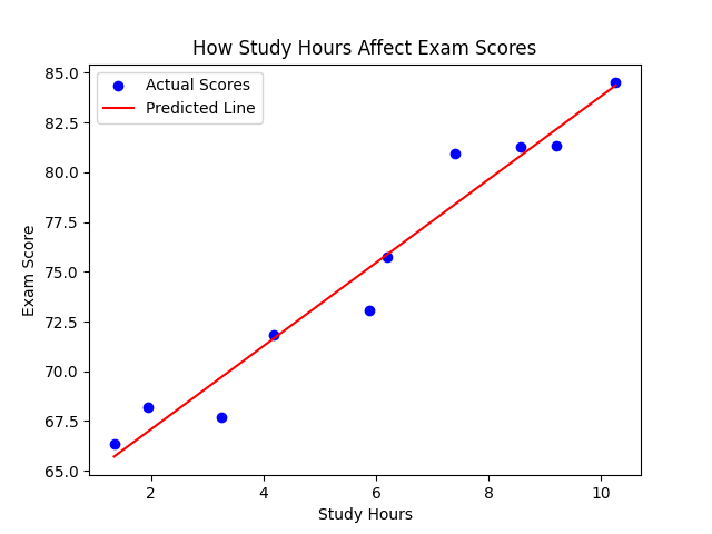
The red line is the model’s prediction and the slope/gradient (e.g., 2.54) means each hour of study adds ~2.5 points to your score. The intercept (e.g., 59.63) is the baseline score if you studied 0 hours.
Real-Life Example: Pizza Sales
Imagine you own a pizza shop. To attract more customers, you decide to give away coupons and eventually, you start to notice that on days when you distribute 50 coupons, you sell 100 pizzas, and on days with 100 coupons, you sell 150 pizzas. You want to find out how many pizzas you would sell if you distributed 500 coupons, so you decide to use your knowledge of linear regression to solve this problem.
Using linear regression, you can create a formula like:
Pizzas Sold = 50 + (1 × Number of Coupons).
This tells you that for every coupon distributed, you sell 1 extra pizza. But even with 0 coupons, you’d still sell 50 pizzas (maybe from regular customers). Now, when you substitute 500 for “Number of Coupons”, you find out that you will be able to sell 550 pizzas.
Common Mistakes to Avoid
- Assuming All Relationships Are Linear:
If your data forms a curve, use polynomial regression instead. - Ignoring Outliers:
A single outlier (e.g., a student who studied 1 hour but scored 90%) can skew the line. - Overcomplicating:
Start with one independent variable (simple regression) before adding more.
Key Takeaways
What: Linear regression predicts a number using a straight-line relationship.
How: Minimize the distance between predicted and actual values.
When: Use linear regression when the relationship between the independent and dependent variables appears linear—meaning that a change in the independent variable results in a proportional change in the dependent variable. It is ideal for forecasting and trend analysis in scenarios where the relationship is stable and straightforward.
Related Reading: